Rasters
Finally we will look at using CSS styling for the portrayal of raster data.

Raster Symbology
Review of raster symbology:
Raster data is Grid Coverage where values have been recorded in a regular array. In OGC terms a Coverage can be used to look up a value or measurement for each location.
When queried with a “sample” location:
- A grid coverage can determine the appropriate array location and retrieve a value. Different techniques may be used interpolate an appropriate value from several measurements (higher quality) or directly return the “nearest neighbor” (faster).
- A vector coverages would use a point-in-polygon check and return an appropriate attribute value.
- A scientific model can calculate a value for each sample location
Many raster formats organize information into bands of content. Values recorded in these bands and may be mapped into colors for display (a process similar to theming an attribute for vector data).
For imagery the raster data is already formed into red, green and blue bands for display.
As raster data has no inherent shape, the format is responsible for describing the orientation and location of the grid used to record measurements.
These raster examples use a digital elevation model consisting of a single band of height measurements. The imagery examples use an RGB image that has been hand coloured for use as a base map.
Reference:
- Raster Symbology (User Manual | CSS Property Listing )
- Rasters (User Manual | CSS Cookbook );
The exercise makes use of the usgs:dem and ne:ne1 layers.
Image
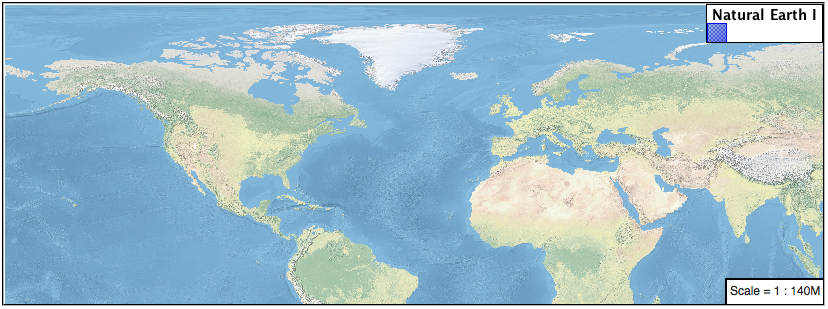
The raster-channels is the key property for display of images and raster data. The value auto is recommended, allowing the image format to select the appropriate red, green and blue channels for display.
Navigate to the CSS Styles page.
Click Choose a different layer and select
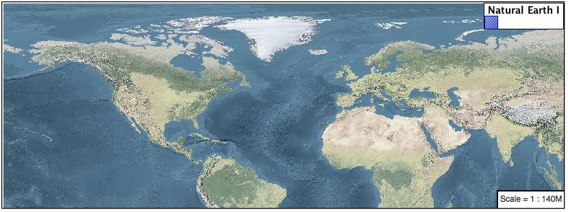
ne:ne1from the list.Click Create a new style and choose the following:
Workspace for new layer: No workspaceNew style name: image_exampleFill in the following css:
* {
  raster-channels: auto;
}
Displaying the unprocessed image:
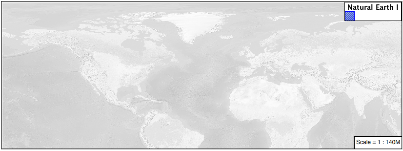
If required a list three band numbers can be supplied (for images recording in several wave lengths) or a single band number can be used to view a grayscale image.
* {
  raster-channels: 2;
}
Isolating just the green band (it wil be drawn as a grayscale image):
DEM
A digital elevation model is an example of raster data made up of measurements, rather than colors information.
The usgs:dem layer used used for this exercise:
From the the CSS Styles page.
Click Choose a different layer and select
usgs:demfrom the list.Click Create a new style and choose the following:
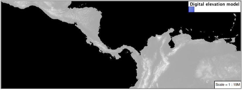
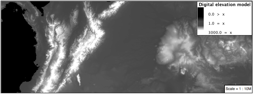
Workspace for new layer: No workspaceNew style name: raster_exampleWhen we use the raster-channels property set to
autothe rendering engine will select our single band of raster content, and do its best to map these values into a grayscale image.* { raster-channels: auto; }
The range produced in this case from the highest and lowest values.
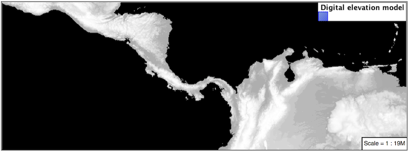
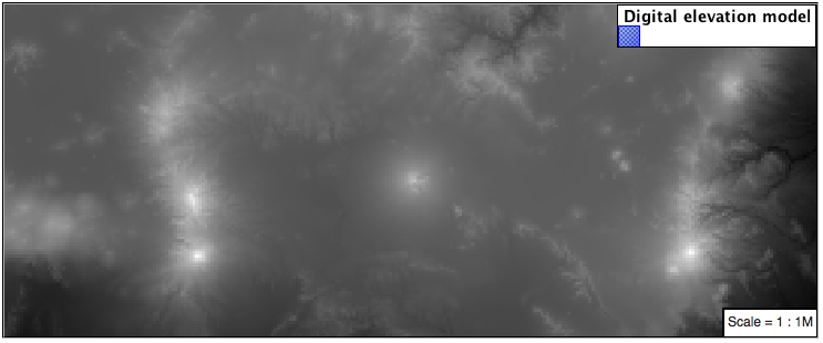
We can use a bit of image processing to emphasis the generated color mapping by making use raster-contrast-enhancement.
* {
  raster-channels: 1;
  raster-contrast-enhancement: histogram;
}
Image processing of this sort should be used with caution as it does distort the presentation (in this case making the landscape look more varied then it is in reality.
Color Map
The approach of mapping a data channel directly to a color channel is only suitable to quickly look at quantitative data.
For qualitative data (such as land use) or simply to use color, we need a different approach:
Apply the following CSS to our usgs:DEM layer:
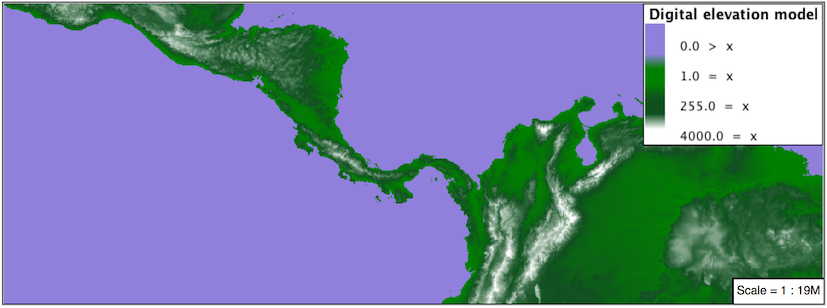
* {
  raster-channels: auto;
  raster-color-map: color-map-entry(#9080DB, 8080)
                    color-map-entry(#008000, 8081)
                    color-map-entry(#105020, 10000)
                    color-map-entry(#FFFFFF, 30000);
}
Resulting in this artificial color image:
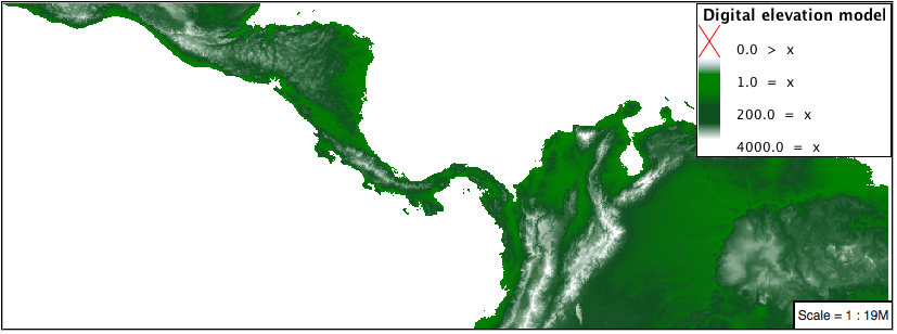
An opacity value can also be used with color-map-entry.
* {
  raster-channels: auto;
  raster-color-map: color-map-entry(#9080DB, 8080, 0.0)
                    color-map-entry(#008000, 8081, 1.0)
                    color-map-entry(#105020, 10000, 1.0)
                    color-map-entry(#FFFFFF, 30000, 1.0);
}
Allowing the areas of zero height to be transparent:
Raster format for GIS work often supply a “no data” value, or contain a mask, limiting the dataset to only the locations with valid information.
Custom
We can use what we have learned about color maps to apply a color brewer palette to our data.
This exploration focuses on accurately communicating differences in value, rather than strictly making a pretty picture. Care should be taken to consider the target audience and medium used during palette selection.
Restore the
raster_exampleCSS style to the following:* { raster-channels: auto; }
Producing the following map preview.
To start with we can provide our own grayscale using two color map entries.
* {
  raster-channels: auto;
  raster-color-map: color-map-entry(#000000, 8080)
                    color-map-entry(#FFFFFF, 30000);
}
Use the Map tab to zoom in and take a look.
This is much more direct representation of the source data. We have used our knowledge of elevations to construct a more accurate style.
While our straightforward style is easy to understand, it does leave a bit to be desired with respect to clarity.
The eye has a hard time telling apart dark shades of black (or bright shades of white) and will struggle to make sense of this image. To address this limitation we are going to switch to the ColorBrewer 9-class PuBuGn palette. This is a sequential palette that has been hand tuned to communicate a steady change of values.
Update your style with the following:
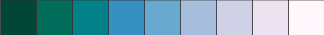
* {
  raster-channels: auto;
  raster-color-map:
     color-map-entry(#014636, 8080)
     color-map-entry(#016c59, 8081)
     color-map-entry(#02818a,10000)
     color-map-entry(#3690c0,15000)
     color-map-entry(#67a9cf,20000)
     color-map-entry(#a6bddb,25000)
     color-map-entry(#d0d1e6,30000)
     color-map-entry(#ece2f0,35000)
     color-map-entry(#fff7fb,40000);
}
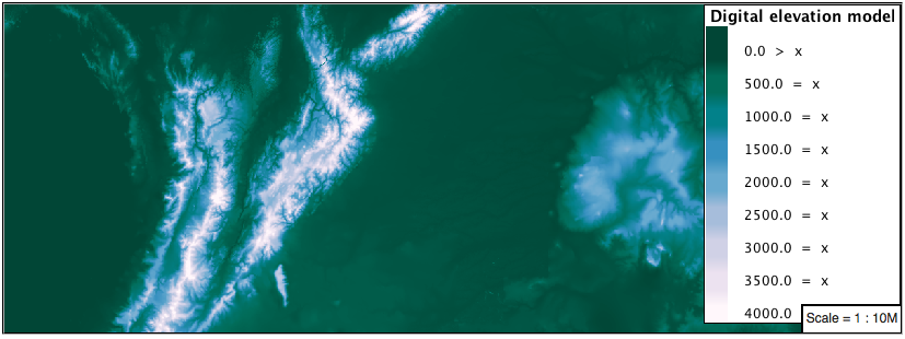
A little bit of work with alpha (to mark the ocean as a no-data section):
* {
  raster-channels: auto;
  raster-color-map:
     color-map-entry(#014636, 8080,0)
     color-map-entry(#016c59, 8081)
     color-map-entry(#02818a,10000)
     color-map-entry(#3690c0,15000)
     color-map-entry(#67a9cf,20000)
     color-map-entry(#a6bddb,25000)
     color-map-entry(#d0d1e6,30000)
     color-map-entry(#ece2f0,35000)
     color-map-entry(#fff7fb,40000);
}
And we are done:
Additional Considerations
Note
This section will contain some extra information related to rasters. If you’re already feeling comfortable, feel free to skip this section.
Automatic Contrast Adjustment
A special effect that is effective with grayscale information is automatic contrast adjustment.
Make use of a simple contrast enhancement with
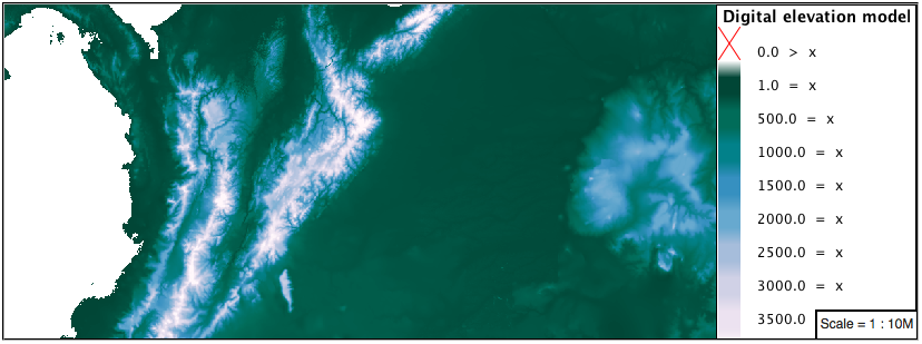
usgs:dem:* { raster-channels: auto; raster-contrast-enhancement: normalize; }
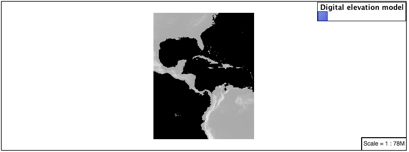
If we zoom in to only show a land area (as indicated with the bounding box below), we will get strange results.
Normalize stretches the palette of the output image to use the full dynamic range. As long as we have ocean on the screen (with value 0) the land area will be shown with roughly the same presentation. Once we zoom in to show only a land area, the lowest point on the screen (say 100) becomes the new black, radically altering what is displayed on the screen.
Color Mapping
The raster-color-map-type property dictates how the values are used to generate a resulting color.
rampis used for quantitative data, providing a smooth interpolation between the provided color values.intervalsprovides categorization for quantitative data, assigning each range of values a solid color.valuesis used for qualitative data, each value is required to have a color-map-entry or it will not be displayed.
We can update our DEM example to use intervals for presentation.
* {
  raster-channels: auto;
  raster-color-map:
     color-map-entry(#014636,   0,0)
     color-map-entry(#014636,   1)
     color-map-entry(#016c59, 500)
     color-map-entry(#02818a,1000)
     color-map-entry(#3690c0,1500)
     color-map-entry(#67a9cf,2000)
     color-map-entry(#a6bddb,2500)
     color-map-entry(#d0d1e6,3000)
     color-map-entry(#ece2f0,3500)
     color-map-entry(#fff7fb,4000);
  raster-color-map-type: intervals;
}
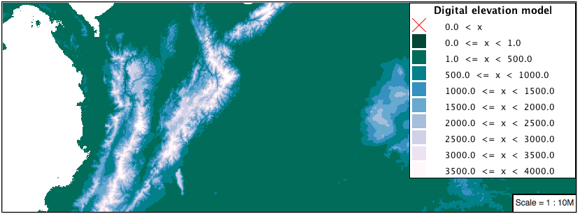
By using intervals it becomes very clear how relatively flat most of the continent is. The ramp presentation provided lots of fascinating detail which distracted from this fact.
Image Processing
Additional properties are available to provide slight image processing during visualization.
Note
In this section are we going to be working around a preview issue where only the top left corner of the raster remains visible during image processing. This issue has been reported as :geos:`6213`.
Image processing can be used to enhance the output to highlight small details or to balance images from different sensors allowing them to be compared.
The raster-contrast-enhancement property is used to turn on a range of post processing effects. Settings are provided for
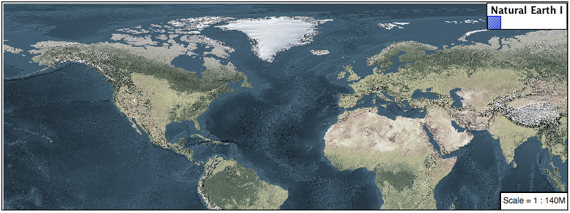
normalizeorhistogramornone;* { raster-channels: auto; raster-contrast-enhancement: normalize; }
Producing the following image:
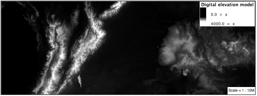
The raster-gamma property is used adjust the brightness of raster-contrast-enhancement output. Values less than 1 are used to brighten the image while values greater than 1 darken the image.
* {
   raster-channels: auto;
   raster-contrast-enhancement: none;
   raster-gamma: 1.5;
}
Providing the following effect:
Mid-tones
In order to present the
ugs:demmore clearly, we can make use of mid-tones. Here is an example css, leaving the oceans dark so the mountains can stand out more.* { raster-channels: auto; raster-color-map: color-map-entry(#000000, 8080) color-map-entry(#444444, 8081) color-map-entry(#FFFFFF, 30000); }
Conclusion
This completes the CSS styling workshop.